Getting Started With Exploratory Data Analysis (EDA)
This notebook serves as a starter guide or template for exploratory data analysis. It will go over the topics mentioned in the EDA guide.
# let's start off by importing the libraries we will need for eda
import pandas as pd
import numpy as np

# for visualizations :
import seaborn as sns
import matplotlib.pyplot as plt
The dataset we will be using in this tutorial is from Analyze Boston. Analyze Boston is the City of Boston’s data hub and is a great resource for data sets regarding the city.
We will be working with the 2022 311 Service Requests dataset. The dataset consists of service requests from all channels of engagement. 311 allows you to report non-emergency issues or request non-emergency City services.
# to run in colab, run the following lines
# from google.colab import drive
# drive.mount('/content/drive')
Mounted at /content/drive
# read in dataset
df = pd.read_csv('311-requests.csv')
pd.set_option('display.max_columns', 6)
# let's look at the first five rows of the dataset
df.head()
| case_enquiry_id | open_dt | target_dt | ... | latitude | longitude | source | |
|---|---|---|---|---|---|---|---|
| 0 | 101004116078 | 2022-01-04 15:34:00 | NaN | ... | 42.3818 | -71.0322 | Citizens Connect App |
| 1 | 101004113538 | 2022-01-01 13:40:13 | 2022-01-04 08:30:00 | ... | 42.3376 | -71.0774 | City Worker App |
| 2 | 101004120888 | 2022-01-09 12:40:43 | 2022-01-11 08:30:00 | ... | 42.3431 | -71.0683 | City Worker App |
| 3 | 101004120982 | 2022-01-09 13:56:00 | NaN | ... | 42.3810 | -71.0256 | Constituent Call |
| 4 | 101004127209 | 2022-01-15 20:42:00 | 2022-01-20 08:30:00 | ... | 42.3266 | -71.0704 | Constituent Call |
5 rows × 29 columns
How many observations/rows are there?
How many variables/columns are there?
What kinds of variables are there? Qualitative? Quantitative? Both?
# number of observations
df.shape[0]
146373
# to see column name, count, and dtype of each column
df.info()
<class 'pandas.core.frame.DataFrame'>
RangeIndex: 146373 entries, 0 to 146372
Data columns (total 29 columns):
 #   Column                          Non-Null Count   Dtype
---  ------                          --------------   -----
 0   case_enquiry_id                 146373 non-null  int64
 1   open_dt                         146373 non-null  object
 2   target_dt                       129475 non-null  object
 3   closed_dt                       125848 non-null  object
 4   ontime                          146373 non-null  object
 5   case_status                     146373 non-null  object
 6   closure_reason                  146373 non-null  object
 7   case_title                      146371 non-null  object
 8   subject                         146373 non-null  object
 9   reason                          146373 non-null  object
 10  type                            146373 non-null  object
 11  queue                           146373 non-null  object
 12  department                      146373 non-null  object
 13  submittedphoto                  55740 non-null   object
 14  closedphoto                     0 non-null       float64
 15  location                        146373 non-null  object
 16  fire_district                   146149 non-null  object
 17  pwd_district                    146306 non-null  object
 18  city_council_district           146358 non-null  object
 19  police_district                 146306 non-null  object
 20  neighborhood                    146210 non-null  object
 21  neighborhood_services_district  146358 non-null  object
 22  ward                            146373 non-null  object
 23  precinct                        146270 non-null  object
 24  location_street_name            145030 non-null  object
 25  location_zipcode                110519 non-null  float64
 26  latitude                        146373 non-null  float64
 27  longitude                       146373 non-null  float64
 28  source                          146373 non-null  object
dtypes: float64(4), int64(1), object(24)
memory usage: 32.4+ MB
There are 146373 rows (observations).
There are 29 columns (variables).
There are both categorical and numerical variables. At quick glance there seems to be more categorical variables than numerical variables.
Categorical Variables: case_status, neighborhood, source, etc.
Numerical Variables: … maybe not?
The case_enquiry_id is a unique identifier for each row, closedphoto has 0 non-null values so it might be worth it to drop this column since there is no additional information we can gather, columns such as location_zipcode, latitude, longitude not exactly numeric varaibles, since they are numbers that represent different codes.
Cleaning
Let’s convert the three time variables (open_dt, target_dt, and closed_dt) from objects to pandas datetime objects. Let’s focus on service requests for a set period of time in 2022. We will start by filtering for service requests that were opened from January 2022 to March 2022.
# changing the three columns with dates and times to pandas datetime object
df['open_dt'] = pd.to_datetime(df['open_dt'])
df['target_dt'] = pd.to_datetime(df['target_dt'])
df['closed_dt'] = pd.to_datetime(df['closed_dt'])

# output is long, but run the line below to check the type of the three columns
#df.dtypes
# filter data for 311 requests from january 2022 to march 2022
df_filtered = df.loc[(df['open_dt'] >= '2022-01-01') &
                  (df['open_dt'] < '2022-03-31')]
df_filtered.head()
| case_enquiry_id | open_dt | target_dt | ... | latitude | longitude | source | |
|---|---|---|---|---|---|---|---|
| 0 | 101004116078 | 2022-01-04 15:34:00 | NaT | ... | 42.3818 | -71.0322 | Citizens Connect App |
| 1 | 101004113538 | 2022-01-01 13:40:13 | 2022-01-04 08:30:00 | ... | 42.3376 | -71.0774 | City Worker App |
| 2 | 101004120888 | 2022-01-09 12:40:43 | 2022-01-11 08:30:00 | ... | 42.3431 | -71.0683 | City Worker App |
| 3 | 101004120982 | 2022-01-09 13:56:00 | NaT | ... | 42.3810 | -71.0256 | Constituent Call |
| 4 | 101004127209 | 2022-01-15 20:42:00 | 2022-01-20 08:30:00 | ... | 42.3266 | -71.0704 | Constituent Call |
5 rows × 29 columns
From our previous observation, since closedphoto column does not contain any non-null values, let’s drop it.
# drop closedphoto column
df_filtered = df_filtered.drop(columns=['closedphoto'])
After filtering the service requests, let’s see how many observations we are left with.
# how many requests were opened from Jan 2022 to March 2022
df_filtered.shape[0]
66520
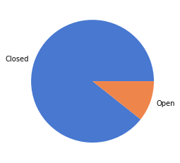
From a quick preview of the dataframe, we can see that some of the requests are still open. Let’s see how many observations are open vs. closed and then how many are ontime vs. overdue from the set of requests from January 2022 to March 2022.
# checking how many open vs. closed cases
df_filtered['case_status'].value_counts()
Closed    59420
Open       7100
Name: case_status, dtype: int64
# visualize case_status in pie chart, set color palette
colors = sns.color_palette('muted')[0:5]
ax = df_filtered['case_status'].value_counts().plot.pie(colors=colors)
ax.yaxis.set_visible(False)
# checking how many ontime vs. overdue cases
df_filtered['ontime'].value_counts()
ONTIME     55089
OVERDUE    11431
Name: ontime, dtype: int64
# visualize ontime in pie chart, set color palette
colors = sns.color_palette('bright')[0:5]
ax = df_filtered['ontime'].value_counts().plot.pie(colors=colors)
ax.yaxis.set_visible(False)

Descriptive Statistics
Pandas makes this easy! We can use describe() to get the descriptive statistics of the numerical columns.
df_filtered.describe()
| case_enquiry_id | location_zipcode | latitude | longitude | |
|---|---|---|---|---|
| count | 6.652000e+04 | 49807.000000 | 66520.000000 | 66520.000000 |
| mean | 1.010042e+11 | 2126.916719 | 42.335694 | -71.075337 |
| std | 3.745629e+04 | 17.188931 | 0.032066 | 0.032259 |
| min | 1.010041e+11 | 2108.000000 | 42.231500 | -71.185400 |
| 25% | 1.010042e+11 | 2119.000000 | 42.314500 | -71.087600 |
| 50% | 1.010042e+11 | 2126.000000 | 42.345900 | -71.062200 |
| 75% | 1.010042e+11 | 2130.000000 | 42.359400 | -71.058700 |
| max | 1.010042e+11 | 2467.000000 | 42.395200 | -70.994900 |
As mentioned before, the case_enquiry_id, location_zipcode, latitude, and longitude columns are not numeric variables. The descriptive statistics are not very useful in this situation.
What would be a useful numeric variable is the duration of a request. Let’s calculate the duration of each of the requests from January 2022 to March 2022 and add it as a new column in our dataframe.
# calculating case duration and adding a new column (case_duration) to the dataframe
duration = df_filtered['closed_dt'] - df_filtered['open_dt']
df_filtered = df_filtered.assign(case_duration=duration)
df_filtered.head()
| case_enquiry_id | open_dt | target_dt | ... | longitude | source | case_duration | |
|---|---|---|---|---|---|---|---|
| 0 | 101004116078 | 2022-01-04 15:34:00 | NaT | ... | -71.0322 | Citizens Connect App | NaT |
| 1 | 101004113538 | 2022-01-01 13:40:13 | 2022-01-04 08:30:00 | ... | -71.0774 | City Worker App | 0 days 03:42:02 |
| 2 | 101004120888 | 2022-01-09 12:40:43 | 2022-01-11 08:30:00 | ... | -71.0683 | City Worker App | 0 days 12:44:07 |
| 3 | 101004120982 | 2022-01-09 13:56:00 | NaT | ... | -71.0256 | Constituent Call | NaT |
| 4 | 101004127209 | 2022-01-15 20:42:00 | 2022-01-20 08:30:00 | ... | -71.0704 | Constituent Call | 0 days 11:36:09 |
5 rows × 29 columns
Now we can see the new case_duration column. Some values are NaT, which means there is a missing date. This makes sense because the case_status is OPEN.
Let’s filter out the open cases and focus on analyzing the duration of the closed cases.
# filter out the open cases
df_closed = df_filtered.loc[(df_filtered['case_status'] == "Closed")]
df_closed.head()
| case_enquiry_id | open_dt | target_dt | ... | longitude | source | case_duration | |
|---|---|---|---|---|---|---|---|
| 1 | 101004113538 | 2022-01-01 13:40:13 | 2022-01-04 08:30:00 | ... | -71.0774 | City Worker App | 0 days 03:42:02 |
| 2 | 101004120888 | 2022-01-09 12:40:43 | 2022-01-11 08:30:00 | ... | -71.0683 | City Worker App | 0 days 12:44:07 |
| 4 | 101004127209 | 2022-01-15 20:42:00 | 2022-01-20 08:30:00 | ... | -71.0704 | Constituent Call | 0 days 11:36:09 |
| 5 | 101004113302 | 2022-01-01 00:36:24 | 2022-01-04 08:30:00 | ... | -71.0587 | Citizens Connect App | 1 days 23:36:53 |
| 6 | 101004113331 | 2022-01-01 03:11:23 | NaT | ... | -71.0587 | Constituent Call | 3 days 05:12:07 |
5 rows × 29 columns
With the closed cases, let’s calculate the descriptive statistics of the new case_duration column.
# let's calculate the descriptive statistics again
# using double brackets to display in a *fancy* table format
df_closed[['case_duration']].describe()
| case_duration | |
|---|---|
| count | 59420 |
| mean | 4 days 12:09:14.466526422 |
| std | 15 days 09:54:44.441079417 |
| min | 0 days 00:00:04 |
| 25% | 0 days 01:26:54.750000 |
| 50% | 0 days 09:01:45 |
| 75% | 1 days 15:40:08.250000 |
| max | 181 days 14:24:23 |
From the table, we can see that the average case duration is ~4.5 days.
The standard deviation for the case duration is ~15.4 days.
The minimum time a case takes to close is 4 minutes.
The maximum time a case takes to close is ~181.6 days.
The inter-quartile range (IQR) is the difference between the 25% and 75% quantiles.
We can also calculate the mode and median.
df_closed['case_duration'].mode()
0   0 days 00:00:54
1   0 days 00:00:57
2   0 days 00:01:03
Name: case_duration, dtype: timedelta64[ns]
df_closed['case_duration'].median()
Timedelta('0 days 09:01:45')
The descriptive statistics summary in table form is nice, but it would be nice to visualize the data in a histogram. Simply trying to plot using the values in the case_duration column will case an error.
Currently, the values in case_duration are of type timedelta64[ns], df_closed['case_duration'] is a Timedelta Series. We will need to apply what is called a frequency conversion to the values.
“Timedelta Series, TimedeltaIndex, and Timedelta scalars can be converted to other ‘frequences’ by dividing by another timedelta, or by astyping to a specific timedelta type.” (See the link below for more information and code examples!)
https://pandas.pydata.org/pandas-docs/stable/user_guide/timedeltas.html
# dividing the case_duration values by Timedelta of 1 day
duration_days = ( df_closed['case_duration'] / pd.Timedelta(days=1))

# adding calculation to dataframe under duration_in_days column
df_closed = df_closed.assign(duration_in_days=duration_days)

# display descriptive statistics summary with new column addition
df_closed[['duration_in_days']].describe()
| duration_in_days | |
|---|---|
| count | 59420.000000 |
| mean | 4.506417 |
| std | 15.413014 |
| min | 0.000046 |
| 25% | 0.060356 |
| 50% | 0.376215 |
| 75% | 1.652873 |
| max | 181.600266 |
# using seaborn library for visualizations
sns.set_theme() # use this if you dont want the visualizations to be default matplotlibstyle
sns.displot(df_closed, x="duration_in_days", binwidth=1)
<seaborn.axisgrid.FacetGrid at 0x16ae584c0>
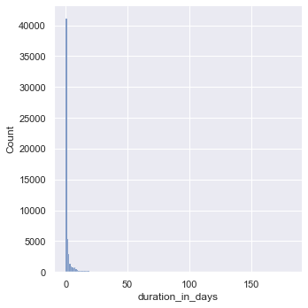
From the plot above, the data seems to be skewed right meaning the right tail is much longer than the left. Let’s try playing with different bin widths.
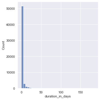
# trying different bin sizes
sns.displot(df_closed, x="duration_in_days", binwidth=5)
<seaborn.axisgrid.FacetGrid at 0x16b031790>
# trying different bin sizes
sns.displot(df_closed, x="duration_in_days", binwidth=25)
<seaborn.axisgrid.FacetGrid at 0x16b06b340>
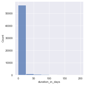
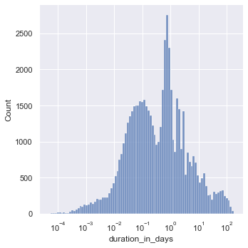
Since the data is heavily skewed, let’s apply log transformation to the data. The log transformation will hopefully reduce or remove the skewness of the original data. The assumption is that the original data follows a log-normal distribution.
# log-scale transformation since the data is heavliy skewed
# add bin_width parameter to change bin sizes
sns.displot(df_closed, x="duration_in_days", log_scale=True)
<seaborn.axisgrid.FacetGrid at 0x16b5577f0>
Which neighborhoods had the most requests from January 2022 - March 2022?
To answer this question, we will take a look at the neighborhood column.
# has 25 unique values so a pie chart probably is not the best option
len(df_closed['neighborhood'].unique())
25
# plot neighborhood counts
sns.countplot(x="neighborhood", data=df_closed).set_title('Number of Requests by Neighborhood')
Text(0.5, 1.0, 'Number of Requests by Neighborhood')
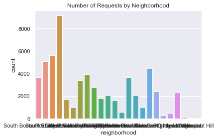
Yikes! The x-axis labels are pretty hard to read. Let’s fix that by plotting the bars horizontally.
# fixing orientation of the labels
sns.countplot(y="neighborhood", data=df_closed).set_title('Number of Requests by Neighborhood')
Text(0.5, 1.0, 'Number of Requests by Neighborhood')
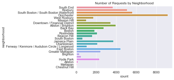
From the plot we can see that Dorchester has the most requests, followed by South Boston/South Boston Waterfront, then Roxbury. There’s a bar that doesn’t have a name…that’s strange. Let’s display the exact counts for each neighborhood.
# displaying number of requests by neighborhood in table form
df_closed['neighborhood'].value_counts()
Dorchester                                      9148
South Boston / South Boston Waterfront          5608
Roxbury                                         5097
East Boston                                     4420
Allston / Brighton                              3945
Jamaica Plain                                   3696
South End                                       3666
Downtown / Financial District                   3419
Back Bay                                        2740
Greater Mattapan                                2429
Hyde Park                                       2308
Charlestown                                     2096
Roslindale                                      2083
Boston                                          1803
West Roxbury                                    1698
Beacon Hill                                     1595
Fenway / Kenmore / Audubon Circle / Longwood    1034
Mission Hill                                     990
South Boston                                     600
                                                 476
Brighton                                         293
Allston                                          141
Mattapan                                          72
Chestnut Hill                                      4
Name: neighborhood, dtype: int64
There are 476 requests without a neighborhood label.
# uncomment and run the line below to check for the empty neighborhood label
# print(df_closed['neighborhood'].unique())

# gather the rows where neighborhood == ' '
df_no_neighborhood = df_closed.loc[(df_closed['neighborhood'] == ' ')]
df_no_neighborhood.head(15) # display first 15 rows
| case_enquiry_id | open_dt | target_dt | ... | source | case_duration | duration_in_days | |
|---|---|---|---|---|---|---|---|
| 163 | 101004115729 | 2022-01-04 11:11:00 | 2022-02-03 11:11:34 | ... | Constituent Call | 0 days 22:32:58 | 0.939560 |
| 207 | 101004117130 | 2022-01-05 14:25:00 | 2022-01-14 14:25:51 | ... | Constituent Call | 35 days 20:34:15 | 35.857118 |
| 301 | 101004118921 | 2022-01-07 12:55:08 | NaT | ... | Constituent Call | 2 days 20:25:31 | 2.851053 |
| 640 | 101004123032 | 2022-01-11 14:00:00 | 2022-01-25 14:00:53 | ... | Constituent Call | 0 days 22:37:49 | 0.942928 |
| 882 | 101004121696 | 2022-01-10 10:35:00 | 2022-01-17 10:35:33 | ... | Employee Generated | 0 days 00:31:04 | 0.021574 |
| 1280 | 101004141822 | 2022-01-20 12:49:51 | 2022-01-31 12:49:51 | ... | Self Service | 0 days 21:40:40 | 0.903241 |
| 1509 | 101004129011 | 2022-01-18 09:11:00 | 2022-02-01 09:11:09 | ... | Constituent Call | 0 days 01:11:18 | 0.049514 |
| 1574 | 101004144874 | 2022-01-24 09:32:51 | 2022-02-07 09:32:51 | ... | Constituent Call | 0 days 00:22:13 | 0.015428 |
| 1612 | 101004146190 | 2022-01-25 12:48:25 | 2022-02-08 12:48:25 | ... | Constituent Call | 0 days 03:36:25 | 0.150289 |
| 1777 | 101004145555 | 2022-01-24 18:24:00 | 2022-02-03 08:30:00 | ... | Constituent Call | 15 days 15:08:31 | 15.630914 |
| 2433 | 101004115813 | 2022-01-04 12:06:54 | 2022-01-06 12:07:26 | ... | Constituent Call | 0 days 02:50:24 | 0.118333 |
| 2489 | 101004116451 | 2022-01-05 02:15:02 | 2022-01-12 08:30:00 | ... | Constituent Call | 0 days 05:25:57 | 0.226354 |
| 2521 | 101004155729 | 2022-01-31 12:20:00 | 2022-02-07 12:21:11 | ... | Employee Generated | 0 days 02:28:06 | 0.102847 |
| 2677 | 101004156474 | 2022-01-31 15:32:00 | 2022-02-14 15:32:53 | ... | Constituent Call | 3 days 02:58:57 | 3.124271 |
| 2687 | 101004156811 | 2022-01-31 16:48:07 | 2022-02-14 16:48:07 | ... | Constituent Call | 0 days 00:03:00 | 0.002083 |
15 rows × 30 columns
print(df_no_neighborhood['latitude'].unique())
print(df_no_neighborhood['longitude'].unique())
[42.3594]
[-71.0587]
The latitude and longitude values are the same for all of the rows without a neighborhood value. We can use the Geopy module to convert the latitude and longitude coordinates to a place or location address - also referred to as reverse geocoding.
# import geopy
from geopy.geocoders import Nominatim

# make a Nominatim object and initialize, specify a user_agent
# Nominatim requires this value to be set to your application name, to be able to limit the number of requests per application
# Nominatim is a free service but provides low request limits: https://operations.osmfoundation.org/policies/nominatim/
geolocator = Nominatim(user_agent="eda_geotest")

# set latitude and longitude and convert to string
lat = str(df_no_neighborhood['latitude'].unique()[0])
long = str(df_no_neighborhood['longitude'].unique()[0])

# get the location information
location = geolocator.reverse(lat + "," +long)

# display location information, add .raw for more details
print(location.raw)
{'place_id': 264213803, 'licence': 'Data © OpenStreetMap contributors, ODbL 1.0. https://osm.org/copyright', 'osm_type': 'way', 'osm_id': 816277585, 'lat': '42.3594696', 'lon': '-71.05880376899256', 'display_name': "Sears' Crescent and Sears' Block Building, Franklin Avenue, Downtown Crossing, Downtown Boston, Boston, Suffolk County, Massachusetts, 02201, United States", 'address': {'building': "Sears' Crescent and Sears' Block Building", 'road': 'Franklin Avenue', 'neighbourhood': 'Downtown Crossing', 'suburb': 'Downtown Boston', 'city': 'Boston', 'county': 'Suffolk County', 'state': 'Massachusetts', 'ISO3166-2-lvl4': 'US-MA', 'postcode': '02201', 'country': 'United States', 'country_code': 'us'}, 'boundingbox': ['42.3593149', '42.3596061', '-71.0592779', '-71.0584887']}
Quick Google Maps search of the location confirms that (42.3594, -71.0587) is Government Center. The output from geopy is Sear’s Crescent and Sears’ Block which are a pair of buildings adjacent to City Hall and City Hall Plaza, Government Center.
Another quick look at the output from geopy shows that the lat and lon values are similar but different from the latitude and longitude values in the dataset.
The requests without a neighborhood value have a general location of Government Center. At least we can confirm that requests without a neighborhood value are not outside of Boston or erroneous.
During January 2022 - March 2022, where did the most case requests come from?
To answer this question, we will take a look at the source column.
# has only 5 unique values so in this case we can use a pie chart
len(df_closed['source'].unique())
5
# displaying the number of requests by each source type
df_closed['source'].value_counts()
Citizens Connect App    32066
Constituent Call        21051
City Worker App          3795
Self Service             1632
Employee Generated        876
Name: source, dtype: int64
# visualizing the breakdown of where case requests come from
# seaborn doesn't have a default pie chart but you can add seaborn color palettes to matplotlib plots

colors = sns.color_palette('pastel')[0:5]
ax = df_closed['source'].value_counts().plot.pie(colors=colors)
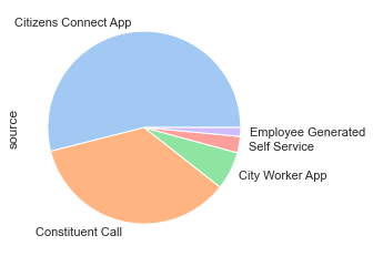
# label each slice with the percentage of requests per source
ax = df_closed['source'].value_counts().plot.pie(colors=colors,autopct='%1.1f%%')

# run the following to remove the default column name label *source*
#ax.yaxis.set_visible(False)
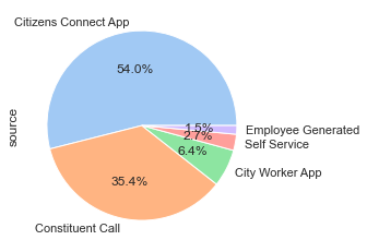
From the pie chart, 54% of the requests from January 2022 - March 2022 came from the Citizens Connect App, 35.4% came from a Constituent Call, followed by 6.4% from the City Worker App.
How many different types of requests were there from January 2022 - March 2022?
To answer this question, we will take a look at the reason column.
# how many different reasons are there
len(df_closed['reason'].unique())
38
# number of requests by reason
df_closed['reason'].value_counts()
Enforcement & Abandoned Vehicles     14908
Code Enforcement                     10437
Street Cleaning                       8477
Sanitation                            5993
Highway Maintenance                   5032
Signs & Signals                       2202
Street Lights                         1774
Recycling                             1690
Housing                               1529
Needle Program                        1298
Building                              1293
Park Maintenance & Safety             1001
Trees                                  762
Animal Issues                          580
Environmental Services                 560
Employee & General Comments            366
Health                                 344
Graffiti                               297
Administrative & General Requests      261
Notification                           141
Traffic Management & Engineering       113
Abandoned Bicycle                      108
Sidewalk Cover / Manhole                53
Catchbasin                              40
Fire Hydrant                            26
Noise Disturbance                       24
Programs                                23
Pothole                                 22
Air Pollution Control                   13
Operations                              11
Neighborhood Services Issues             9
Weights and Measures                     8
Cemetery                                 7
Generic Noise Disturbance                7
Parking Complaints                       5
Fire Department                          3
Office of The Parking Clerk              2
Billing                                  1
Name: reason, dtype: int64
There were 38 different types of requests from January 2022 - March 2022, the top three with most requests being Enforcement & Abandoned Vehicles with 14,908 requests, Code Enforcement with 10,437 requests, then Street Cleaning with 8,477 requests.
# top case request reason by neighborhood
df_closed.groupby(['neighborhood'])['reason'].describe()
| count | unique | top | freq | |
|---|---|---|---|---|
| neighborhood | ||||
| 476 | 17 | Employee & General Comments | 278 | |
| Allston | 141 | 17 | Code Enforcement | 29 |
| Allston / Brighton | 3945 | 31 | Enforcement & Abandoned Vehicles | 1065 |
| Back Bay | 2740 | 29 | Enforcement & Abandoned Vehicles | 678 |
| Beacon Hill | 1595 | 23 | Street Cleaning | 467 |
| Boston | 1803 | 30 | Enforcement & Abandoned Vehicles | 378 |
| Brighton | 293 | 21 | Enforcement & Abandoned Vehicles | 64 |
| Charlestown | 2096 | 27 | Enforcement & Abandoned Vehicles | 766 |
| Chestnut Hill | 4 | 3 | Health | 2 |
| Dorchester | 9148 | 32 | Enforcement & Abandoned Vehicles | 2195 |
| Downtown / Financial District | 3419 | 28 | Enforcement & Abandoned Vehicles | 807 |
| East Boston | 4420 | 27 | Enforcement & Abandoned Vehicles | 1935 |
| Fenway / Kenmore / Audubon Circle / Longwood | 1034 | 28 | Enforcement & Abandoned Vehicles | 202 |
| Greater Mattapan | 2429 | 27 | Sanitation | 546 |
| Hyde Park | 2308 | 28 | Sanitation | 431 |
| Jamaica Plain | 3696 | 28 | Code Enforcement | 819 |
| Mattapan | 72 | 16 | Street Cleaning | 19 |
| Mission Hill | 990 | 25 | Enforcement & Abandoned Vehicles | 208 |
| Roslindale | 2083 | 30 | Enforcement & Abandoned Vehicles | 387 |
| Roxbury | 5097 | 30 | Enforcement & Abandoned Vehicles | 1019 |
| South Boston | 600 | 19 | Enforcement & Abandoned Vehicles | 243 |
| South Boston / South Boston Waterfront | 5608 | 27 | Enforcement & Abandoned Vehicles | 2530 |
| South End | 3666 | 27 | Code Enforcement | 775 |
| West Roxbury | 1698 | 24 | Sanitation | 450 |
# get counts for each request reason by neighborhood
reason_by_neighborhood = df_closed.groupby(['neighborhood', 'reason'])['duration_in_days'].describe()[['count']]
reason_by_neighborhood
| count | ||
|---|---|---|
| neighborhood | reason | |
| Cemetery | 7.0 | |
| Code Enforcement | 9.0 | |
| Employee & General Comments | 278.0 | |
| Enforcement & Abandoned Vehicles | 17.0 | |
| Environmental Services | 3.0 | |
| ... | ... | ... |
| West Roxbury | Signs & Signals | 95.0 |
| Street Cleaning | 159.0 | |
| Street Lights | 50.0 | |
| Traffic Management & Engineering | 4.0 | |
| Trees | 72.0 |
594 rows × 1 columns
# run this cell to write the reason by neighborhood to a csv to see all rows of data
reason_by_neighborhood.to_csv('reasons_by_neighborhood.csv')
# let's take a look at the South End neighborhood specifically
south_end_df = df_closed.loc[(df_closed['neighborhood'] == 'South End')]
south_end_df.groupby(['reason'])['duration_in_days'].describe()[['count']]
| count | |
|---|---|
| reason | |
| Abandoned Bicycle | 8.0 |
| Administrative & General Requests | 10.0 |
| Air Pollution Control | 4.0 |
| Animal Issues | 16.0 |
| Building | 52.0 |
| Code Enforcement | 775.0 |
| Employee & General Comments | 1.0 |
| Enforcement & Abandoned Vehicles | 712.0 |
| Environmental Services | 48.0 |
| Fire Hydrant | 2.0 |
| Graffiti | 55.0 |
| Health | 8.0 |
| Highway Maintenance | 360.0 |
| Housing | 40.0 |
| Needle Program | 269.0 |
| Neighborhood Services Issues | 1.0 |
| Noise Disturbance | 2.0 |
| Notification | 2.0 |
| Park Maintenance & Safety | 73.0 |
| Recycling | 29.0 |
| Sanitation | 242.0 |
| Sidewalk Cover / Manhole | 1.0 |
| Signs & Signals | 76.0 |
| Street Cleaning | 717.0 |
| Street Lights | 118.0 |
| Traffic Management & Engineering | 7.0 |
| Trees | 38.0 |
What types of cases typically take the longest to resolve?
To answer this question, let’s take a look at the duration_in_days and reason columns.
# what types of cases typically take the longest
# case_duration by reason

sns.catplot(x="reason", y="duration_in_days", kind="box", data=df_closed,)
<seaborn.axisgrid.FacetGrid at 0x16ba4bf10>
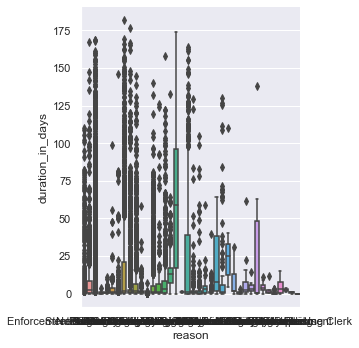
# The chart is kind of difficult to read...
# Let's fix the size of the chart and flip the labels on the x-axis

sns.catplot(y="reason", x="duration_in_days", kind="box", data=df_closed,
            height = 8, aspect = 1.25)
<seaborn.axisgrid.FacetGrid at 0x16bfc04c0>
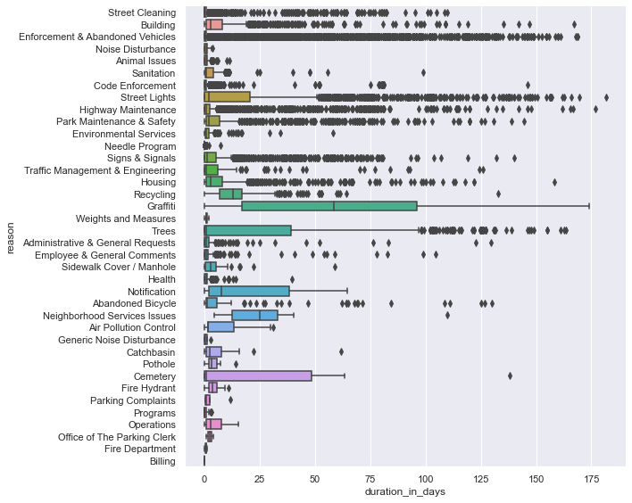
Box plots display the five-number-summary, which includes: the minimum, the maximum, the sample median, and the first and third quartiles.
The box plot shows the distribution duration_in_days in a way that allows comparisions between case reasons. Box plots show the distribution of a numerical variable broken down by a categorical variable.
The box shows the quartiles of the duration_in_days and the whiskers extend to show the rest of the distribution (minimum and maximum). Points that are shown outside of the whiskers are determined to be outliers. The line inside the box is the median.
# descriptive statistics for duration_in_days by case reason
# box plot in table form
pd.set_option('display.max_columns', None)
df_closed.groupby(['reason'])['duration_in_days'].describe()
| count | mean | std | min | 25% | 50% | 75% | max | |
|---|---|---|---|---|---|---|---|---|
| reason | ||||||||
| Abandoned Bicycle | 108.0 | 15.100783 | 30.637974 | 0.005799 | 0.610787 | 1.154815 | 5.827731 | 129.944907 |
| Administrative & General Requests | 261.0 | 3.812869 | 13.899890 | 0.000081 | 0.114005 | 0.781192 | 1.984132 | 129.670035 |
| Air Pollution Control | 13.0 | 8.872239 | 10.842552 | 0.001528 | 1.787616 | 1.790822 | 13.153194 | 30.967199 |
| Animal Issues | 580.0 | 0.904125 | 1.086867 | 0.000127 | 0.075793 | 0.705457 | 1.238536 | 11.121447 |
| Billing | 1.0 | 0.009178 | NaN | 0.009178 | 0.009178 | 0.009178 | 0.009178 | 0.009178 |
| Building | 1293.0 | 8.183306 | 16.727784 | 0.000046 | 0.642755 | 2.649641 | 8.094919 | 167.316273 |
| Catchbasin | 40.0 | 6.295217 | 10.713959 | 0.000174 | 0.946927 | 2.444572 | 7.476412 | 61.852523 |
| Cemetery | 7.0 | 33.686310 | 52.072679 | 0.000127 | 0.113744 | 0.594907 | 48.409045 | 138.163553 |
| Code Enforcement | 10437.0 | 0.646142 | 3.440879 | 0.000069 | 0.054375 | 0.234653 | 0.752095 | 146.231354 |
| Employee & General Comments | 366.0 | 3.045888 | 11.407637 | 0.000243 | 0.050307 | 0.607309 | 1.707879 | 104.725579 |
| Enforcement & Abandoned Vehicles | 14908.0 | 4.326244 | 17.119537 | 0.000058 | 0.057263 | 0.177986 | 0.620069 | 168.863750 |
| Environmental Services | 560.0 | 1.750664 | 3.612940 | 0.000069 | 0.500052 | 0.870752 | 1.994499 | 57.933796 |
| Fire Department | 3.0 | 0.598248 | 0.542678 | 0.001887 | 0.365845 | 0.729803 | 0.896429 | 1.063056 |
| Fire Hydrant | 26.0 | 4.028460 | 2.648591 | 0.000914 | 2.174317 | 3.593819 | 5.515179 | 10.837072 |
| Generic Noise Disturbance | 7.0 | 0.809901 | 1.071081 | 0.000498 | 0.010162 | 0.476505 | 1.120243 | 2.931493 |
| Graffiti | 297.0 | 60.795557 | 44.483313 | 0.000278 | 16.802164 | 58.580428 | 95.905475 | 173.824433 |
| Health | 344.0 | 1.524580 | 3.127143 | 0.000058 | 0.143215 | 0.894028 | 1.253898 | 39.648924 |
| Highway Maintenance | 5032.0 | 4.621423 | 14.838073 | 0.000081 | 0.070668 | 0.775781 | 2.315587 | 176.714560 |
| Housing | 1529.0 | 7.676885 | 14.967539 | 0.000058 | 0.692222 | 2.935729 | 8.104514 | 158.114988 |
| Needle Program | 1298.0 | 0.079918 | 0.243719 | 0.000081 | 0.017248 | 0.029554 | 0.053157 | 7.152766 |
| Neighborhood Services Issues | 9.0 | 31.791151 | 31.721388 | 4.324954 | 12.663229 | 24.884931 | 32.983403 | 109.890347 |
| Noise Disturbance | 24.0 | 0.909435 | 1.072071 | 0.000104 | 0.005830 | 0.614433 | 1.358082 | 3.525995 |
| Notification | 141.0 | 19.565133 | 20.603048 | 0.000544 | 1.802569 | 7.719329 | 38.391088 | 64.423113 |
| Office of The Parking Clerk | 2.0 | 2.440463 | 2.261498 | 0.841343 | 1.640903 | 2.440463 | 3.240023 | 4.039583 |
| Operations | 11.0 | 4.725810 | 5.460231 | 0.000266 | 0.697992 | 2.894306 | 7.657731 | 15.175023 |
| Park Maintenance & Safety | 1001.0 | 10.480097 | 21.813287 | 0.000347 | 0.710787 | 1.846771 | 6.700729 | 144.606782 |
| Parking Complaints | 5.0 | 3.200009 | 4.912111 | 0.387477 | 0.388090 | 0.889826 | 2.483206 | 11.851447 |
| Pothole | 22.0 | 3.910974 | 3.141983 | 0.001771 | 1.924826 | 3.009109 | 5.652931 | 14.102245 |
| Programs | 23.0 | 0.658821 | 1.055246 | 0.000336 | 0.001233 | 0.056863 | 0.813414 | 3.142951 |
| Recycling | 1690.0 | 12.245377 | 9.035924 | 0.000081 | 6.856282 | 12.930035 | 16.928313 | 132.917153 |
| Sanitation | 5993.0 | 2.403129 | 3.185305 | 0.000058 | 0.260671 | 0.979294 | 3.836354 | 98.852222 |
| Sidewalk Cover / Manhole | 53.0 | 4.735583 | 8.858981 | 0.000127 | 0.358148 | 2.873461 | 5.035451 | 58.847674 |
| Signs & Signals | 2202.0 | 6.620529 | 14.839239 | 0.000185 | 0.143718 | 1.167795 | 5.073134 | 140.114028 |
| Street Cleaning | 8477.0 | 1.082891 | 6.127272 | 0.000046 | 0.037975 | 0.100706 | 0.605370 | 109.824236 |
| Street Lights | 1774.0 | 18.585520 | 32.664829 | 0.000104 | 0.148079 | 1.984855 | 20.707622 | 181.600266 |
| Traffic Management & Engineering | 113.0 | 11.388050 | 25.003672 | 0.000729 | 0.085231 | 0.842176 | 6.080509 | 125.919988 |
| Trees | 762.0 | 25.210341 | 41.285189 | 0.000139 | 0.018481 | 0.804022 | 39.169418 | 163.697106 |
| Weights and Measures | 8.0 | 0.985169 | 0.558955 | 0.107234 | 0.741134 | 0.900399 | 1.207185 | 1.808912 |
Graffiti cases take on average take the longests time to resolve, 60.796 days.
Do cases typically take longer in one neighborhood over another?
# do cases typically take longer in one neighborhood over another?

sns.catplot(y="neighborhood", x="duration_in_days", kind="box", data=df_closed,
            height = 8, aspect = 1.25)
<seaborn.axisgrid.FacetGrid at 0x16c38f880>
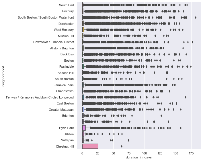
The box plot above shows several outliers for each category (neighborhood) making it difficult to read and quite overwhelming.
Let’s display the information in table form.
# in table form
df_closed.groupby(['neighborhood'])['duration_in_days'].describe()
| count | mean | std | min | 25% | 50% | 75% | max | |
|---|---|---|---|---|---|---|---|---|
| neighborhood | ||||||||
| 476.0 | 4.178610 | 13.672122 | 0.000127 | 0.058209 | 0.705318 | 2.208099 | 138.163553 | |
| Allston | 141.0 | 3.947410 | 9.929540 | 0.000058 | 0.134988 | 0.873414 | 2.763426 | 63.832847 |
| Allston / Brighton | 3945.0 | 4.622345 | 14.786827 | 0.000185 | 0.075984 | 0.511424 | 1.995000 | 161.749630 |
| Back Bay | 2740.0 | 4.900469 | 16.733563 | 0.000197 | 0.043553 | 0.215110 | 1.172946 | 166.873588 |
| Beacon Hill | 1595.0 | 2.485273 | 10.776832 | 0.000301 | 0.042506 | 0.167801 | 0.863617 | 136.561204 |
| Boston | 1803.0 | 5.152869 | 17.959729 | 0.000046 | 0.041944 | 0.345833 | 1.555781 | 156.934120 |
| Brighton | 293.0 | 5.162394 | 14.575959 | 0.000266 | 0.078623 | 0.547211 | 2.031343 | 126.706586 |
| Charlestown | 2096.0 | 4.147373 | 14.840357 | 0.000081 | 0.067653 | 0.278171 | 1.162135 | 139.983704 |
| Chestnut Hill | 4.0 | 19.075249 | 30.039288 | 0.148611 | 0.185148 | 6.448744 | 25.338845 | 63.254896 |
| Dorchester | 9148.0 | 3.956899 | 12.579649 | 0.000046 | 0.068087 | 0.515260 | 1.883400 | 156.208553 |
| Downtown / Financial District | 3419.0 | 3.475034 | 13.957725 | 0.000231 | 0.050648 | 0.234988 | 0.973443 | 176.714560 |
| East Boston | 4420.0 | 2.777781 | 10.877246 | 0.000058 | 0.037833 | 0.181094 | 0.902786 | 150.815174 |
| Fenway / Kenmore / Audubon Circle / Longwood | 1034.0 | 7.722932 | 19.772496 | 0.000150 | 0.101777 | 0.636291 | 2.556918 | 165.773264 |
| Greater Mattapan | 2429.0 | 4.807563 | 14.036534 | 0.000104 | 0.084375 | 0.678646 | 2.818472 | 158.114988 |
| Hyde Park | 2308.0 | 6.664146 | 16.259478 | 0.000127 | 0.081476 | 0.747078 | 5.331976 | 157.788715 |
| Jamaica Plain | 3696.0 | 6.216330 | 18.281044 | 0.000104 | 0.081823 | 0.569161 | 2.147717 | 148.726493 |
| Mattapan | 72.0 | 3.742091 | 11.557064 | 0.000069 | 0.071858 | 0.725631 | 2.012494 | 74.130579 |
| Mission Hill | 990.0 | 5.582632 | 18.433571 | 0.000081 | 0.055107 | 0.281186 | 1.690460 | 137.808854 |
| Roslindale | 2083.0 | 7.048947 | 21.030090 | 0.000289 | 0.109369 | 0.714190 | 2.658108 | 173.824433 |
| Roxbury | 5097.0 | 5.020254 | 17.307327 | 0.000069 | 0.070324 | 0.495382 | 1.817338 | 161.948993 |
| South Boston | 600.0 | 3.175501 | 14.327518 | 0.000058 | 0.055269 | 0.228287 | 1.015081 | 159.967488 |
| South Boston / South Boston Waterfront | 5608.0 | 3.160470 | 14.300232 | 0.000150 | 0.051296 | 0.181863 | 0.827731 | 181.600266 |
| South End | 3666.0 | 4.225789 | 16.643360 | 0.000243 | 0.043921 | 0.187778 | 0.967399 | 167.869965 |
| West Roxbury | 1698.0 | 6.004628 | 17.783995 | 0.000081 | 0.106288 | 0.787685 | 3.035735 | 161.054688 |
In January 2022 - March 2022, cases took the longest in Chestnut Hill. Cases typically lasted on average 19.075 days but there were only 4 cases located in Chestnut Hill during this time. Smaller sample sizes could mean more variability (look at standard deviation to explain the spread of observations).
We can further look at the population of Chestnut Hill versus the other neighborhoods to try and make sense of this low case count. Additionally, we can broaden the time period of the cases to see if Chestnut Hill still has a low case count.
From the table above we can see how long cases take by each neighborhood, it would be interesting to further breakdown by case reason for each neighborhood.
Wrap Up, Next Steps
Further analysis could be done using the 311 dataset. Using the 311 data from previous years, we can see how number of requests have changed over the years, or how case duration may have changed over the years.
Since most requests have latitude and longitude coordinates it could be interesting to plot each case request on a map to see if there are clusters of requests in certain locations.
Next steps could include gathering demographic data to overlay on top of the 311 dataset for further analysis. Another possible next step would be to build a model to predict how long a request could take given the request reason, subject, location, source, etc.
Click here to download this Jupyter Notebook (make sure you are signed in with your BU email)!